
SPICE: Sparsity Promoting Iterated Constrained Endmember Extraction Algorithm
Problem Statement: Hyperspectral Data Collection
Need an intro about Hyperspectral Imaging? Check out our HyperspectralAnalysisIntroduction repository.
Hyperspectral cameras (HSCs) provide a huge contribution to remote sensing data. They have been used in a variety of application such as food safety, biomedical, and forensic applications. HSCs are operated on specific regions of the electromagnetic spectrum. Some are focused on the VNIR and others on SWIR. Below is an example of how Hysperspectral Image (HSI) looks like:
There are many aspects in Hyperspectral imaging (HSI) that would affect the gathered data by the sensors, like atmospheric effects, light scattering to different molecules before reflected back to the sensor, and many other. In addition, some pixels would have a wide field of view where each pixel would be a 1x1 meter or even higher in reality. Pixels with this size could have multiple objects in them. For example, disregarding atmospheric effects, a pixel could have sand, water, and bricks in it and when the sensor captures the reflectance, the spectrum of that pixel will be a mix of those 3 materials. That is why it would be hard to tell if the spectra that is being observed is a pure pixel of the object being analyzed because it could be a mix of other materials in that field. Therefore, each pixel needs to be decomposed into multiple special spectra called endmembers. There are many mixing model algorithms in the state-of-the-art. This article will discuss the Linear Mixing Model (LMM). The LMM assumes that each pixel is a mix of spectra that consists of endmembers and a proportion value for each endmember. Multiplying each proportion value with its corresponding endmember and adding them up will produce the seen spectrum. Below is the LMM equation.
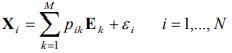
$N$ is the number of pixels in the image, $M$ is the number of endmembers, $\mathbf{X}i$ is the observed pixel, $p{ik}$ is the proportion of endmember $k$ in pixel $i$, $\boldsymbol{E}k$ is the $k{th}$ endmember, and $\varepsilon_i$ is an error term. The LMM assumes that each of the 3 materials, from the previous example, has its own endmember and a proportion value for each endmember in every pixel and combing them produces the seen spectrum. The figure below illustrates this process for a single pixel captured by HSC.
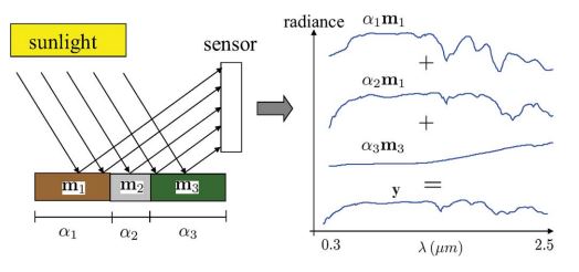
where y represents the measured spectrum for that pixel (it is the Xi in the LMM equation). The m (it is the Ek in the LMM equation) represents the endmembers and in this case, there are 3 endmembers. Etimating the number of endmembers present in an HSI data is known as Hyperspectral Unmixing. Endmembers are an estimated representative spectra of the materials in HSI. From the pixel example mentioned previously, each of the sand, water, bricks will have their own endmember.
There are many endmember extraction algorithms in the state-of-the-art with a variety of approaches like geometrical, statistical, and sparse regression (Bioucas-Dias, et. al., 2012). This post is about Sparsity Promoting Iterated Constrained Endmember Extraction algorithm also known as SPICE, which is a geometrical approach of finding the endmembers
Method: SPICE
To put it in the most simple manner, take the figure below as an example for how the LMM equation works (disregrading the error term).
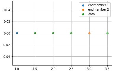
This is a one-dimensional example. The endmembers are already defined and substituting the values into LMM using x as random data point:
p1×1+p2×3=x
which provides an equation with 2 unknown variables. There needs to be another equation to solve the system of equations. Therefore, the SPICE algorithm includes a constraint that says the value of each proportion should be ≥0 and the sum of the proportions for each data should equal to 1.
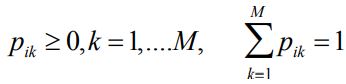
This constraint will make sure that the data is inside the region that the endmembers cover. Now the system can be solved for p1 and p2 using this constraint.
p1+3p2=x
p1+p2=1
which will yields
p1=3-x⁄2
p2=x-1⁄2
substituting 1.5, for example, as a data point:
p1=0.75
p2=0.25
Another example, using 3.5 as the data point will yield:
p1=-0.25
p2=1.25
which violates the constraint that the proportion values must be ≥0 and would produce an error. This is how the constraint is making sure the data is inside the region that the endmembers cover.
Another example in 2D is shown below.
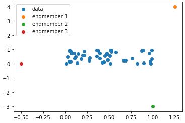
.JPG)
When the endmembers are connected, it will create a simplex (triangle) shape, which is the region that the data should be inside of.
The data needs to be inside the canvas that the endmembers create, which is why the SPICE algorithm includes a constraint that the value of each proportion should be positive and the sum of the proportions for each data should equal to 1.
where p is the proportion and M is the number of endmembers. Here is another example with 2D data. As mentioned before, the data needs to be inside the region that the endmembers create when connecting them together. In the example below if the endmembers are connected, it will create a simplex (triangle) shape.
The same concept applies, the closer the data to an endmember, the higher the proportion of that data will be to that endmember and the rest of the proportions will be divided to the other endmembers. In cases where the data is placed outside of the simplex, this will result in an error. A solution to this error could be adding an extra endmember to expand the simplex region to include that data. This brings in the concept of how SPICE does not actually have a unique solution. Meaning, from the triangle example above, there are infinite number of ways to include this whole data using 3 endmembers. It can also be done using more than 3 endmembers. So there are 2 problems that needs to be addressed:
- Minimize the error between the data and estimated endmembers to decrease the number of endmembers.
- Minimize the distance between the endmembers to have the smallest region as possible coverd by the endmembers or find a tight fit around the data.
How is the error between the data and estimated endmembers minimized?
The error between the data and estimated endmembers is minimized using the residual sum of squared formula.
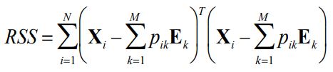
where Xi is the data, p is the proportion, and Ek is the endmember. The equation is minimized subjected to the contraint mentioned previously.
How is the distance between the estimated endmembers minimized?
The distance between the estimated endmembers is minimized using the sum of squared distance formula.
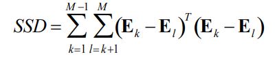
The equation is minimized subjected to the contraint mentioned previously.
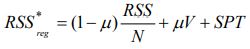
The objective function
Implementation of SPICE
SPICE is implemented using the following steps:
- Random number of endmembers are initialized (could also be initialized to a random set of data)
- The proportions are calculated from the endmembers by minimizing the Quadratic Programming Problem (QPP).
- New members are found based on the proportions from step 2 using the below equation.
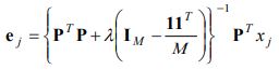
- steps 2 and 3 are iteratively repeated until the objective function RSSreg is smaller than a threshold value.
Applications of SPICE
Check Out the Code and Paper!
This work was accepted to the SPIE. Digital Library! Our code is available!
Citation
Plain Text:
A. Zare and P. Gader, “SPICE: a sparsity promoting iterated constrained endmember extraction algorithm with applications to landmine detection from hyperspectral imagery,” in Proc. SPIE 6553, Detection and Remediation Technologies for Mines and Minelike Targets XII, 2007.
BibTex:
@InProceedings{zare2007spice,
Title = {SPICE: a sparsity promoting iterated constrained endmember extraction algorithm with applications to landmine detection from hyperspectral imagery},
Author = {Zare, Alina and Gader, Paul},
Booktitle = {Proc. SPIE 6553, Detection and Remediation Technologies for Mines and Minelike Targets XII},
Year = {2007},
Month = {Apr.},
Number = {655319},
Volume = {6553},
Doi = {10.1117/12.722595}}
Links


![]()